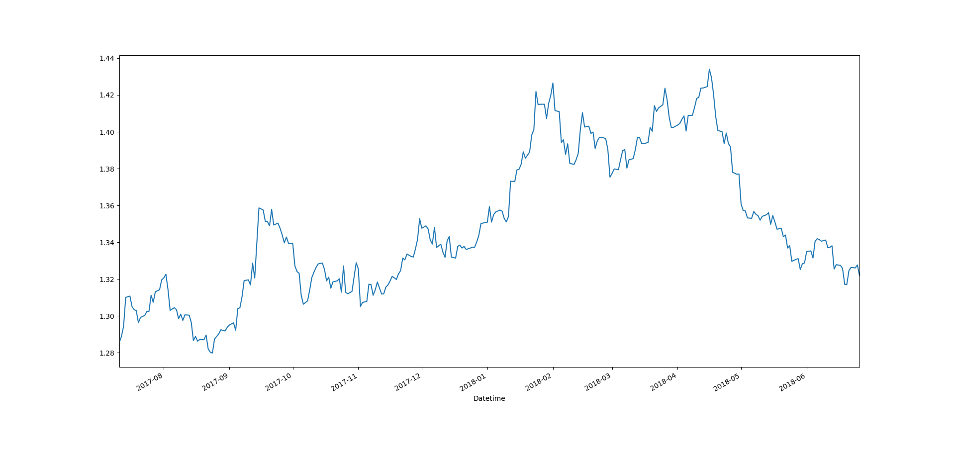
Dynamic Linear Models were first used in the Apollo space program. Later on in the Polaris aerospace program and Voyager spacecraft orbit determination, oceanographic problems, agriculture, economics speech recognition and many more. In the last three decades Dynamic Linear Models also known as DLM have found widespread use in diverse fields like biology, environment, quality control, engineering, economics, finance and of course trading. You might have heard about the Kalman Filter. Kalman Filter is a basic DLM. DLMs are linear models that assume Gaussian distribution for the innovations or errors. When we assume Gaussian, we can use a Kalman Filter to solve the DLM in a recursive manner. In reality, financial market returns are not Gaussian at all rather financial time series show fat tail behavior. To solve the fat tail problem, Particle Filters got developed. Particle Filters are widely used now a days in algorithmic trading. But before we start developing our own particle filters, you will have to master Dynamic Linear Models. Below is a daily closing price of GBPUSD. As you can see this is a non stationary time series and cannot be dealt with the traditional ARIMA models.
In this post I will focus on DLMs. We will be discussing how to build and use dynamic linear models (DLM) in your trading strategies. Algorithmic trading is all about building predictive models. If we have a good predictive model, we can build a trading strategy around it. We can use machine learning in building predictive models. Models are based on your assumptions and hence are a subjective thing based on your experiences. What this means is that the derived forecast is just a hypothesis and a conjecture about the future. So there is a great possibility that the derived forecast is wide off the mark giving a sizable predictive error. Now when using a dynamic linear model, it is precisely these forecasting errors that are used by the system for learning and improving performance. Keep this in fact I believe we can develop a dynamic linear model for price that can learn from its past forecasting errors and improve upon it. Did you read the post on how to trade with Triple Exponential Moving Average?
If you have been frustrated by the poor ARIMA model price forecasts, then you should stop despairing now. DLMs are much better than ARIMA models when it comes to modeling non stationary time series like price. DLMs are much more flexible as compared to ARIMA models when it comes to modeling non stationary time series with structural changes. DLMs basically try to model the observation time series as being driven by a hidden state variable also known as latent variable. We can model ARIMA as a DLM special case. So DLMs are more flexible and versatile as compared to ARIMA models. The thing most advantageous is that DLMs are sequential models meaning we can do computations recursively. This is very important when we have to make predictions in real time for algorithmic trading. Read the post on can we predict Flash Crashes with LSTM Recurrent Neural Network Model.
We have incomplete information about the financial markets. We don’t know the variables that drive the price. We can say we have general idea how the price gets determined but most of the time we get shocked when the market surprises us by behaving in a totally unpredictable manner. So the basic questions in modeling price boils down to how we are going to deal with imperfect information at our disposal. One information that we have is the values of the financial time series values as it evolves over time. How do we deal with uncertainty? We deal with uncertainty by using probabilities. This is what we do we assign probabilities to the different parameters in our model. These probabilities are mostly subjective and are derived from expert knowledge. Read the post on Fuzzy Hammer Candlestick Pattern Indicator.
In this post my aim will be to explain how to build such a dynamic linear model for forecasting price after n bars and then use is practically in our trading system. Just keep this in your mind. Modelling is an art. Good modelling needs hard thinking. Good forecasting requires an integrated view of the system. Dynamic linear models allow us to use Bayesian statistics which is something really useful. Bayesian statistics treats all uncertainty as a probability distribution. The biggest uncertainty that we face while trading is will our stop loss get hit and if the stop loss doesn’t get hit luckily than whether the profit target will be hit or not. The purpose of building models is to forecast both the risk as well as the profit target and see if we have a good forecast.
In Bayesian forecasting all probabilities are subjective and represent the beliefs of the modeler. We will be basically dealing with financial time series OHLC (Open, High, Low and Close). Most of the time we will use the closing price. Let’s denote price with the generic variable $Y$ and the financial time series developing as $Y_1, Y_2, Y_3, Y_4……Y_t$. $1,2,3,4…t$ denote the observations at the different time interval starting from $1$ and ending at $t$. Now there is not special need for the time intervals to be equally spaced but most of the time we will assume the time intervals to be equally spaced. In dynamic linear models we assume that the probability distribution of the random variables is normal. Read the post on can we use regression splines in day trading?
Dynamic Linear Model Observation And System Equations
We start at time ${0}$. Information available at time ${0}$ is $D_0$. Information available at time $t$ will be $D_t$. Forecasting ahead to time $s > t$ requires the forecasting distribution for $(Y_s|D_t)$. As time evolves we receive more information that can help us in improving about predictions. So at time $t$ the information $D_t=\lbrace Y_t, D_{t-1} \rbrace$. The information is being received sequentially. Building a forecasting model requires making some assumptions which are known as model parameters $\theta$ rather $\theta_t$ as the model parameters also evolve through time. At time $t$, historical information $D_{t-1}$ is summarized through a prior distribution. The prior density $p(\theta_t | D_{t-1})$ and the posterior density $$p(\theta_t | D_t)$$ provide a concise formula for the information traveling with the time series data generating process through time. A dynamic linear model is represented by the quadruple $ \lbrace F_t, \lambda , V_t , W_t \rbrace $:
Observation Equation: $Y_t=F_t\mu_t+\nu_t $ $\nu_t \sim N[0,V_t]$
System Equation: $\mu_t=\lambda\mu_{t-1}+\omega_t$ $\omega_t \sim N[0,W_t]$
Initial Information: $ \mu_0 | D_0\sim N[m_0,C_0]$
These are the basic dynamic linear model equations. All we need to do is choose the mean and variance of the initial information in the initial information equation and the observation variance $V_t$ and the system variance $W_t$. We most of the time use the maximum likelihood estimation to estimate these model parameters. There are many interesting DLMs that we can make from the above basic dynamic linear model equations.
First Order Polynomial Model
First order polynomial is the simplest DLM that is popular. The observation equation is $Y_t=\mu_t+\nu_t $ $\nu_t \sim N[0,V_t]$ where $\mu_t$ is the level of the time series at time t and $\nu_t$ is the observation error which is normally distributed. The local level $\mu_t$ evolves as a simple random walk $\mu_t=\mu_{t-1}+\omega_t$ $\omega_t \sim N[0,W_t]$. Now we can also model the observation and evolution equations as $(Y_t | \mu_t) \sim N[\mu_t, V_t]$ and $(\mu_t | \mu_{t-1} \sim N[\mu_{t-1},W_t]$. In this model, local level is fairly constant apart from random fluctuations in the short term but is variable in the long run. So if you forecast k steps ahead, the expected forecast will be $E[Y_{t+k}]=\mu_t$. You must have guessed right. First order polynomial model is not suitable for forecasting price k steps ahead as it will just forecast the present level. The forecast function $f_t (k) = m_t$ meaning it is a constant. This is only useful for very short term predictions and as said above it is not suitable for forecasting price n bars ahead.
e are studying this model as it is a simple model and studying it will help us understand more complicated models that I am going to discuss below. The one step ahead forecast for this model is:
Posterior for $\mu_{t-1}$: $(\mu_{t-1}|D_{t-1} \sim N[m_{t-1}, C_{t-1}]$
Prior for $\mu_t$: $\mu_t |D_{t-1} \sim N[m_{t-1}, R_t]$
where $R_t=C_{t-1}+W_t$
First step forecast: $(Y_t|D_{t-1})\sim N[m_t, C_t]$
where $f_t=m_{t-1}$ and $Q_t=R_t+V_t$
Posterior for $\mu_t$: $(\mu_t|D_t)\sim N[m_t, C_t]$
As said again and again, we are interested in building a model that can provide us with reliable forecasts that we can use in building our algorithmic trading system. The two main forecast distributions for us are the marginals $(Y_{t+k}|D_t)$$ and $$(X_t(k)|D_t)$ where $X_t(K)=Y_{t+1}+Y_{t+2}+……Y_{t+k}$. First is known as the k step ahead forecast and the second k step lead time forecast.
The Random Walk Plus Noise Model
The constant level model is characterized by $\lbrace 1,1,V,W \rbrace$. The ratio $r=\dfrac{W}{V}$ is known as the Signal to Noise Ratio that you will hear a lot in signal processing papers.The information set $D_t=\lbrace Y_t, D_{t-1}$ does not contain any external information. This type of model that does not contain any external information is known as a Closed Model. Closed Model is not a good model as it does not allow us to consider extra external information that might help us improve the k step ahead forecasts. It is just not acceptable in building a predictive model that ignores extra external information that can help us.
Bayesian statistics allow us to combine subjective information and model/data information. This is precisely one of the major reasons why we want to build a Bayesian Dynamic Linear Model for forecasting price k steps ahead. This will be particularly helpful when making predictions before FOMC Meeting Minutes Release, NFP Report Release and other major events that happen off and on like the Brexit and ECB Press Conferences etc. When using this constant model for predicting stock prices, currency prices and commodity prices, appropriate value for observation variance V may be close to zero as compared to the system variance W.
Discounting Information Decay In Financial Markets
At this stage we should bring in the concept of Discount Factor. Information decays in the financial markets. Recent information is more relevant as compared to information a few weeks old. In the above model the we have both observation variance $V$ and the system variance $W$ constant. Using a discount factor we can let the information decay sequentially. Choosing discount factor $\delta$ between $0.8$ and $1$ does this trick. So we have this relationship $W_t=C_{t-1}\dfrac{1-\delta}{\delta}$.
Using the above relation linking the system variance with the observation variance through the discount factor, we only have to make a guess for observation variance $$V_t$$ which is most of the time unknown. In the constant model we have $V_t=V$. Often we use $\phi=\dfrac{1}{V}$ where $\phi$ is known as Precision. We will focus on this constant model and try to build a currency trading forecasting model based on it. Using the discount factor helps us decay the information at a constant rate or constant rate of increase of uncertainty. So using discount factor we don’t have a constant model but quickly converges to the constant DLM $\lbrace 1,1,V, rV \rbrace$ where $r=\dfrac {(1-\delta)^2}{\delta}$. As you can see now, we only need to know $$V$$ for starting the constant DLM. Model building is all an art and a skill involving many things that are subjective. This is what we can do build a number of models and then combine their predictions into a one forecast. Each model will have its own forecast. We can weigh the forecasts and combine them into a one.
In financial time series prediction, the observable process is more important as compared to the latent process and we are more interesting in forecasting. The parameters in the model like $V_t $ and $W_t$ are to be estimated before we can make the forecasting. Dynamic Linear Models are also known as Gaussian State Space Models. Just keep in mind DLMs are special cases of general State Space Models. Learn how to easily download intraday stock data from Google Finance.
Local Linear Trend Model Or The Linear Growth Model
Local Linear Trend Model is more elaborate as compared to the Random Noise plus Noise Model where we assumed that time series mean was a random walk. In local linear trend model we assume that the slope of the mean is varying with time. This adds another random variable in our DLM and makes it more complex.
$Y_t=\mu_t+\nu_t $
$\nu_t \sim N[0,V]$
$\mu_t=\mu_{t-1}+\beta_{t-1}+\omega_{t1}$
$\omega_{t1} \sim N[0,\sigma_{\mu}^2]$
$\beta_t=\beta_{t-1}+\omega_{t2}$
$\omega_{t2} \sim N[0,\sigma_{\beta}^2]$
The three errors $\nu_t, \omega_{t1}$ and $\omega_{t2}$ are uncorrelated. Now this is a DLM according to the definition that gave above with:
$\theta_t=\begin{pmatrix}
\mu_t \\
\beta_t
\end{pmatrix}$
$G=\begin{pmatrix}
1 & 1 \\
0 & 1
\end{pmatrix}$
$W=\begin{pmatrix}
\sigma_{\mu}^2 & 0 \\
0 & \sigma_{\beta}^2
\end{pmatrix}$
$F=\begin{pmatrix}
1\\
0
\end{pmatrix}$
The matrices $F_t$, $G_t$ and the covariance matrices $V_t$ and $G_t$ are constants so the local linear trend model is time invariant. Linear Trend Model can be used in building a price forecasting system. In the above model we have assume time invariant parameters for the model. First we try that and check the forecasts. After that we improve the model by including time varying parameters. But that would introduce too much complexity in the model. If you have read my post carefully you would have learned something known as discounting information decay. We can introduce a discounting factor in the model and see whether the forecasts improve or not. Did you check my Million Dollar Trading Challenge? The purpose of Million Dollar Trading Challenge is to help others traders and start with $200 and turn that into a million dollar in less than 12 months.
Linear Growth Model is basically a second order polynomial DLM. Polynomial order DLM models higher than three are very rare. So the local linear trend model is a second order polynomial model. At any time $t$, the second order polynomial DLM has a straight line forecast function $f_t(k)=a_{t0}+a_{t1}k$. Now as you can see the forecasting function is a straight line. If you try a local linear trend, the straight line can be steep meaning pretty soon the forecasts are way beyond what is possible. As I had said, one way to overcome the forecast function to have a steep slope is to use a discount factor that will ensure that forecasts don’t become too unrealistic.
Now there are two approaches to applying the discount factor. One is to discount the trend $\mu_t$ and the growth $\beta_t$ separately. But the better approach is to apply a single discount factor to the local linear trend model as a whole with this $W_t=\dfrac{1-\delta}{\delta}L_2C_{t-1}L_2^T$. As I said, discounting allows the information to decay with more weight given to the recent observations. As you can see the discounting is being done through the parameter values. This is unlike the exponential smoothing that is applied to the price time series.
The Third Order Polynomial DLMs
A third order polynomial DLM has the forecast function $f_t(k)=a_{t0}+a_{t1}k+a_{t2}k^2$. As you can see the forecast function for the third order polynomial DLM is a quadratic function. Most of the time second order polynomial DLM or the local linear trend model will be adequate to model the closing price. Quadratic Growth Model is another name for the third order polynomial model.
$ Y_t=\mu_t+\nu_t$
$\mu_t=\mu_{t-1}+\beta_t+\partial\mu_t$
$\beta_t=\beta_{t-1}+\gamma_t+\partial\beta_t$
$\gamma_t=\gamma_{t-1}+\partial\gamma_t$
Above is the Quadratic Growth model. In the continuous time case, $\beta_t$ would be the first derivative of the mean level of the time series and the $\gamma_t$ would be the second derivative of the expected mean level of the price time series. As said, higher order polynomial DLMs greater than three are very rare. As said above, our main purpose is price prediction. Yesterday, there was a surprise jump by GBPUSD when Germany announced that it was ready to accept a less detailed agreement in order to get the Brexit deal done. This news was bullish for GBPUSD and it jumped straight 100 pips. Can we predict such a move? Let’s check with by building a Quadratic Growth Model. I like Quadratic Growth Model better as compared to Linear Trend Model as it involves both a slope and the growth factor. Let’s build a simple Quadratic Growth Model using R.
library(dlm)
data1 <- read.csv("D:/Shared/MarketData/GBPUSD240.csv",
                  header=FALSE)
colnames(data1) <- c("Date", "Time", "Open", "High", "Low",
                     "Close", "Volume")

#number of rows
x1 <- nrow(data1)
quotes1 <- as.ts(data1$Close)
#define k
k <- 1
y <- quotes1[(x1-225):(x1-k)]


# set up SS model
buildQuadGrowth <- function(parm){
  parm <- parm_rest(parm)
  dlm <- dlmModPoly(3,dV=1e-7,dW=c(0,0,0))

  return( dlm )
}

# estimate parameters
fit <- dlmMLE(y, parm=rep(0,3), buildQuadGrowth)
fit$convergence
fit$par


nAhead <-25
dlmPrice <- buildQuadGrowth(fit7$par)
filterDLM <- dlmFilter(c(y, rep(NA, nAhead)), mod =dlmPrice)
tail(filterDLM$f, nAhead)
In the above model, I have taken the system variances as zero and the observation variance as 1e-7. These are standard assumptions made when building local linear trend and growth models. I have used GBPUSD 240 minute data and made predictions for the next 25 bars. The predictions are:
> tail(filterDLM$f, nAhead)
 [1] 1.291248 1.291449 1.291653 1.291861 1.292071 1.292285 1.292501 1.292721 1.292944
1.293169 1.293398 1.293630 1.293865 1.294103
[15] 1.294344 1.294588 1.294835 1.295085 1.295338 1.295594 1.295853 1.296116 1.296381
1.296649 1.296921
Now I have posted the screenshot of GBPUSD H4 chart below.
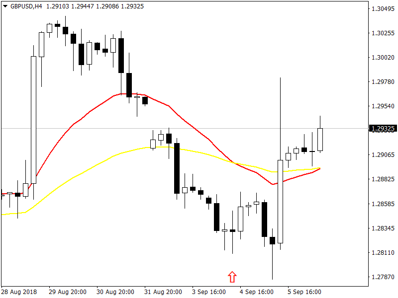
Red arrow shows the point where we are making predictions. As you can see price immediately did not jump up. First it went down to the level 1.27847 then it jumped. Our Quadratic Growth Model is predicting price to immediately jump up after the red arrow. If we run the model with GBPUSD 60 minute data we get the following predictions:
> tail(filterDLM$f, nAhead)
 [1] 1.278205 1.278060 1.277915 1.277770 1.277625 1.277480 1.277335 1.277190 1.277045
1.276900 1.276755 1.276610 1.276465 1.276320
[15] 1.276175 1.276031 1.275886 1.275741 1.275596 1.275451 1.275306 1.275161
1.275016 1.274871 1.274726
You can see the model is predicting the price to go down on 60 minute timeframe. Now these models are very crude. They cannot be used in trading in the present form right now. What I was checking was whether the DLMs that I am building do have the predictive power? You can see the DLMs on different time frames do have the predictive power. We need to refine them and then combine them in a model pipeline that can be used in building an algorithmic trading system. The next step will be of course to use discounting in our model and see if we have improvement in our forecasts. After that we should develop a few autoregressive DLMs with constant as well as time varying parameter and see what can we forecasts. Why we need to build different models? Why one model is not going to work is because markets are too complicated and one model cannot predict the market all the time accurately. In the end, we need to select the best models and combine them into a one using Bayesian machine learning. Did you read the post on can LSTM model could have predicted GBPUSD flash crash?
Local Linear Trend Model With Discount Factor
When we build models, we should use the Occam’s Razor. Simple models should be preferred over more complicated models. No model will be accurate 100% but simple models can solve the problem and at the same time be computationally less intensive. We need a simple trading model that is robust and can reliably adapt to changing market conditions. In the above R code, I have used DLM library. DLM library is a robust library and can do a lot of Bayesian modelling. You should read the book,”Dynamic Linear Models with R” by Sonia Petrone and Giovanni Petris. You should also read the book,”Bayesian Forecasting and Dynamic Models” by Harrison and West. The idea of discounting information in a dynamic model has been discussed by Harrison and West in their book. Sonia and Giovanni have picked the idea from them and developed a simple discounting filter that we are now going to use and see if we get what we want meaning forecasting accuracy.
#Local Linear Trend DLM model
library(dlm)
source("DLM/Rfunctions/DLMFilterDF.R")
# Import the csv file
data1 <- read.csv("D:/Shared/MarketData/GBPUSD240.csv",
                  header=FALSE)
colnames(data1) <- c("Date", "Time", "Open", "High", "Low",
                     "Close", "Volume")

#number of rows
x1 <- nrow(data1)
quotes1 <- as.ts(data1$Close)
#define k
k <- 1
y <- quotes1[(x1-325):(x1-k)]
# set parameter restrictions (only variances here)
parm_rest <- function(parm){
  return( c(exp(parm[1]),exp(parm[2]), exp(parm[3])) )
}

localTrend <- function(parm){
  parm <- parm_rest(parm)
  dlm1 <- dlm(FF = matrix(c(1, 0), nr = 1),
              V = parm[1],
              GG = matrix(c(1, 0, 1, 1), nr = 2),
              W = diag(c(0, parm[2])),
              m0 = rep(0, 2),
              C0 = parm[3]* diag(2))

  return(dlm1)
}


fit <- dlmMLE(y, parm=rep(0.1,3), localTrend)
fit$convergence
fit$par


dlmPrice <- localTrend(fit$par)

#filter the price and forecast
nAhead <-25
filterDLM <- dlmFilter(c(y, rep(NA, nAhead)), mod =dlmPrice)
filterDLM <- dlmFilterDF(c(y, rep(NA, nAhead)), mod =dlmPrice,
                         DF=0.95)
tail(filterDLM$f, nAhead)
#tail(data1,25)
plot(y)
lines(as.ts(filterDLM$f), col='red')
There is a special function available on the website of Dynamic Liner Models with R. I have used this function dlmFilterDF. We have a dynamic linear model with unknown state vector and unknown parameters. In the case of local linear trend model, we have unknown observation variance matrix and the state covariance matrix also known as evolution matrix. If we don’t use discounting of information, the local linear trend model make the following predictions for the next 6 H4 bars:
> tail(filterDLM$f, nAhead)
[1] 1.281011 1.279744 1.278478 1.277211 1.275945 1.274679
You can see above the general direction of the market has been picked correctly by the local linear trend model. It’s just that it is unable to tell us that price touched 1.28700 before it fell down. Let’s check with the discounting factor in the local linear trend model. When we use the local linear trend model with discount factor, we can only make the next one step ahead prediction. This is due to the fact that the predictive distribution is a Student-t distribution instead of the Normal distribution in the case of simple local linear trend model. I will explain the reasons in detail below. First let’s see what we get:
> tail(filterDLM$f, nAhead)
[1] 1.288636       NA       NA       NA       NA       NA
I used the discounting factor of 0.95 and the next bar close is predicted to be 1.28863. The actual close was 1.28556. I used 0.95 as a discount factor. I could have used 0.9 as the discount factor. There is no way for us to guess what discounting factor the market is using. So a good idea is to use two discount factors and average the predictions. If we use 0.9 as the discount factor the predicted closing price for the next H4 candle is 1.28336 and if we average these two predictions we get 1.28599. So we are pretty close. Price infact made a high of 1.28700 and then closed at 1.28556. So you can see now with your own eyes using discounting factor in the local linear trend model has made it pretty effective. I cannot quote the detailed formulas you can check them in these two books but when we have a DLM with unknown parameter we have a Normal Gamma prior as the conjugate density. When we have a Normal Gamma as the filtering distribution, the predictive distribution is a Student-t distribution. Student-t distribution is a much better predictive distribution as compared to the Normal distribution when it comes to predicting financial markets. This is due to the fact the Student-t distribution has more heavy tail as compared to the Normal distribution.
State Covariance Matrix $W_t$ has a crucial role in determining the role of past observations in making state estimation and forecasting. If you check the above code, in our Local Linear Trend State Covariance Matrix $W_t$ is a diagonal matrix. Large diagonal values means high uncertainty in the state evolution and as a result a lot of sample information is thereby lost when we make estimation from $\theta_{t-1}$ to $\theta_t$. Actually this is what is happening. We have sample information $y_1:y_{t-1}$ which are used to estimate $\theta_{t-1}$. When we move from $\theta_{t-1}$ to $\theta_t$ most the sample information is lost and the model relies heavily on $y_t$ in making the prediction. If you check above, local linear trend without discounting made the prediction of 1.28101 for the next H4 bar closing price which is almost the same as the last closing price in our sample. $R_t=P_t+W_t$ is the variance of the forecasting distribution. As you can see $W_t$ is increasing the uncertainty or what we call the variance. If we express $W_t=\dfrac{1-\delta}{\delta}P_t$ we can reduce the uncertainty. This is how we can reduce the uncertainty in the model by using the discount factor.
Problem with DLMs
DLMs have one major problem? Guess what? Yes it is the Gaussian assumption. The underlying probability distribution is assumed to be normal or what we call Gaussian. What we need is a predictive model that is Non Gaussian. We can do that by building a particle filter. In the particle filter the underlying probability distribution is Non Gaussian. What we build here we improve with the particle filter so we haven’t wasted out time. Regularly read my Day Trade Blog. In this post I have build a local linear tend model with discounting and used it to predict the next H4 candle. In the future post, we will remove the assumption of Gaussian distribution in our Local Linear Trend Model and develop a Particle Filter Model that estimates the underlying distribution from the sample data. But still you can see with a pretty simple tweak to the DLM, we have been able to improve the forecasting. This simple tweak is the concept of discount factor. We will need this discount factor in particle filtering as well as this concept is crucial when it comes to information decay in the financial markets.
In nutshell a trading model is a mathematical representation of the dynamics driving the market. As long as your trading model and the underlying market are in synchronization, the trading model will keep on predicting the market correctly. When the market changes, the synchronization between the trading model and the market will break and the trading signals generated by the model will stop giving good predictions. So we need a mechanism that can judge the synchronization between the market and the trading model. In future posts I will dwell on that as well so keep on reading my blog regularly and I will be happy to answer your comments if you have any.
I am revisitng this post once again. In this post I posted coded on how to discount the system variance $W$. I didn’t discuss how to discount the observation variance $V$. In the near future, I will post the code for how to discount the observation variance $V$ so stay tuned. The big problem is knowing at what rate the market is discounting information. A discount factor of 1 means 100% information is being passed to the next observation while a discount factor of 0.9 means only 90% of the information is being passed to the future while 10% of the information is being lost. Now you should keep this in mind, financial time series such as the closing price time series is not normally distributed rather is heavy tailed. Let’s fit Quadratic Growth Model to GBPUSD Weekly data.
filterDelta <- function(x){
filterDLM <- dlmFilterDF(c(y,rep(NA, nAhead)),
mod =dlmPrice, DF=x)
#res1 <- residuals(filterDLM, sd=FALSE)
#return (c(filterDLM$f[length(y)+1], res1[length(y)]))
return (c(filterDLM$f[length(y)+1]))
}
fun1 <- function(x){
  filterDelta(x)-quotes1[x1-k+1]
}
uniroot(fun1,c(0.5,1))$root
#delta1 <-sapply(delta, filterDelta)
#plot(delta, delta1)
#plot(delta, delta1[1, ])
#plot(delta, delta1[2, ])


#0.8306938
#0.9659784
#0.9718284
#0.9811853
#0.9843826
#0.9974674
#0.9961071
Above you can see that the discount factor is changing with each observation. Discount factors like 0.99 are indicative of the Quadratic Growth Model being a good fit to the data. Discount factor like 0.83 indicates that the Quadratic Growth Model is not a good fit. Actual problem is how to find the discount factor for predicting the next observation. Below is the Quadratic Growth Model fit to the GBPUSD weekly day for the discount factor of 0.993724.
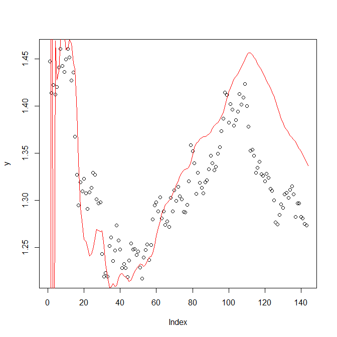
As you can see from the above chart, the model is not fitting in the last part. Since we are using Maximum Likelihood Estimation (MLE) for the estimation of model parameters and MLE is heavily dependent on the length of the window which means the number of observations we use to do the estimation. Another method can be using Markov Chain Monte Carlo. More on that below. In the beginning the Kalman Filter took some time to adjust then it slowly started following the data. As I said above, each observation requires a new discount factor as the market is continuously changing the rate at which it is discounting information. We need to find a reliable method to find the appropriate discount factor. One method can be to take a look at the residuals of the model and analyze the residuals.
> filterDLM <- dlmFilterDF(c(y, rep(NA, nAhead)), mod =dlmPrice, + DF=0.993724)
> res <- residuals(filterDLM, sd=FALSE)
> #res <- residuals(filterDLM, sd=TRUE)
> MAD <- sum(abs(res[1:length(y)]))/length(y) > MAD
[1] 3.460074
> MSE <- sum(res[1:length(y)]^2)/length(y) > sqrt(MSE)
[1] 4.410729
> qqnorm(res)
> tsdiag(filterDLM)
> plot(y)
> lines(as.ts(filterDLM$f), col='red')
> library(forecast)
> checkresiduals(res)
Warning message:
In modeldf.default(object) :
  Could not find appropriate degrees of freedom for this model.
Model One Step Ahead Prediction Error Analysis
One step ahead prediction errors are very important for us. DLM model can easily calculate the one step ahead prediction errors for each observation. When we have large one step ahead prediction errors it means the model is not working. A discount factor is only valid for one observation as the market keeps on changing at which rate it discounts the information. First let’s check the qqnorm plot this is the QQ plot of the residuals against the normal distribution. QQ plot is used for testing whether the error distribution is normal or not. In case of a perfect fit the QQ norm would be a 45 degree straight line.
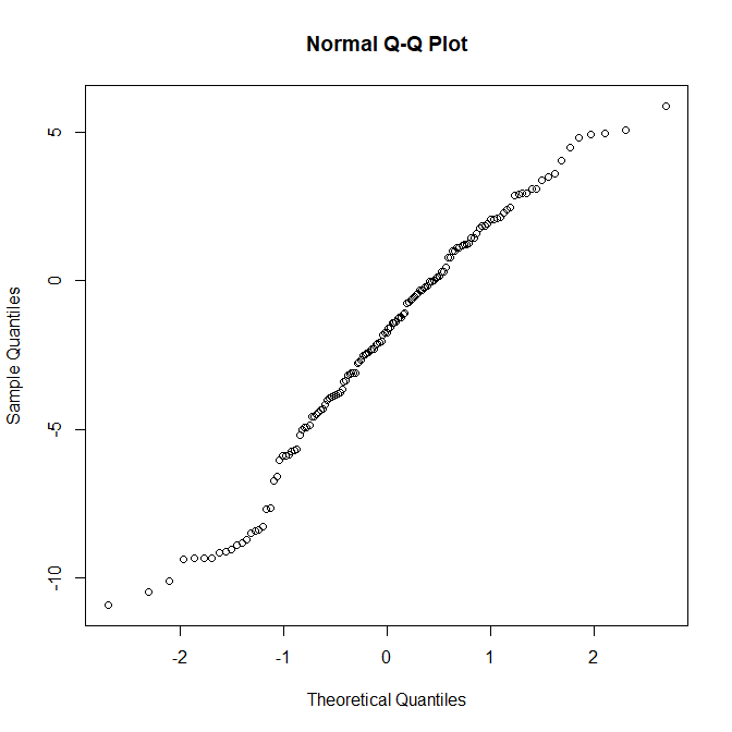
As you can see in the above QQ plot, the residuals are not normal at all. Let’s diagnose more. Below are the screenshots of the residual diagnosis. As you can see the residuals are heavily correlated and the model in the last stages is clearly out of sync with the observed data.
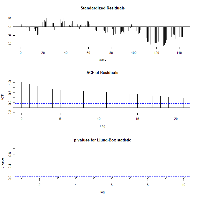
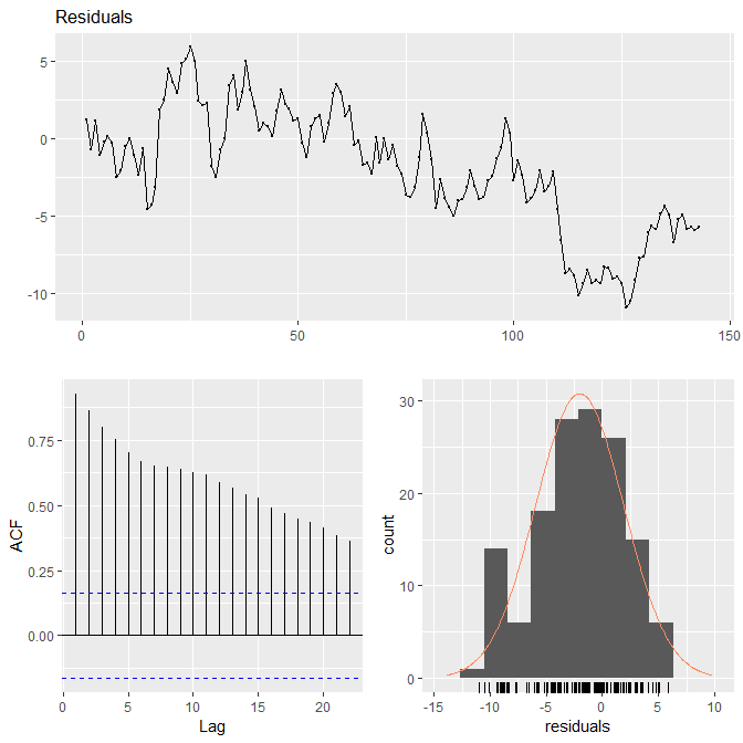
As you can see the residuals are correlated. Let’ use R forecast library to analyze the residuals. You can see in the Residuals plot below the residuals or one step ahead prediction errors are wide off the mark after observation 100. This is a clear sign that the model has broken and is not fitting well for this discount factor. As I said above, each observation needs a new discount factor.
This plot has been made using the forecast library. Take a look at my Million Dollar Trading Challenge.
Markov Chain Monte Carlo Gibbs Sampler
As said above one method of model parameter estimation is the MLE which is a robust method but has limitations. Another method that we can use to estimate the model parameters is Markov Chain Monte Carlo (MCMC) Gibbs Sampling. I wont go into the details of MCMC Gibbs Sampling. Gibbs Sampling is a popular method in Bayesian analysis.
> k <- 9 > y <- quotes1[(x1-100):(x1-k)]
> MCMC <- 12000
> gibbsOut <- dlmGibbsDIG(y, mod = dlmModPoly(3),
+ a.y = 1, b.y = 1000, a.theta = 1, b.theta = 1000,
+ n.sample = MCMC, thin = 1, save.states = FALSE)
> burn <- 2000
> mcmcMean(gibbsOut$dV[-(1 : burn)])
  gibbsOut$dV[-(1:burn)]
  1.04e-04
 (4.08e-07)
> mcmcMean(gibbsOut$dW[-(1 : burn)])
  gibbsOut$dW[-(1:burn)]
  1.83e-04
 (2.13e-05)
> # set parameter restrictions (only variances here)
> parm_rest <- function(parm){ + return( c(exp(parm[1]),exp(parm[2]), exp(parm[3]))) + } >
> quadraticGrowth <- function(parm){
+   parm <- parm_rest(parm)
+   dlm1 <- dlm(FF = matrix(c(1, 0, 0), nr = 1),
+ V = parm[1], + GG = matrix(c(1, 0, 0, 1, 1, 0, 0, 1, 1),
+ nr = 3), + W = diag(c(0, 0, parm[2])),
+ m0 = rep(0, 3), + C0 = parm[3]* diag(3))
+
+ return(dlm1)
+ }
>
>
>
> fit <- dlmMLE(y, parm=rep(0,3), quadraticGrowth, debug=FALSE)
There were 14 warnings (use warnings() to see them)
> fit$convergence
[1] 0
> fit$par
[1]  -9.3114204 -11.0530113  -0.7161337
> fit$par[1] <-log(mcmcMean(gibbsOut$dV[-(1 : burn)])[1])
> fit$par[2] <-log(mcmcMean(gibbsOut$dV[-(1 : burn)])[2])
>
> dlmPrice <- quadraticGrowth(fit$par)
>
> #filter the price and forecast
> nAhead <-1
> filterDLM <- dlmFilter(c(y, rep(NA, nAhead)), mod =dlmPrice, + debug=FALSE)
> tail(filterDLM$f, nAhead)
[1] 1.262035
You can see Gibbs Sampling has improved the situation. The advantage of Gibbs Sampling is that we are less dependent on window size ( number of observations). Let’s check the residuals now after plugging in the Gibbs Sampler estimated parameter values.
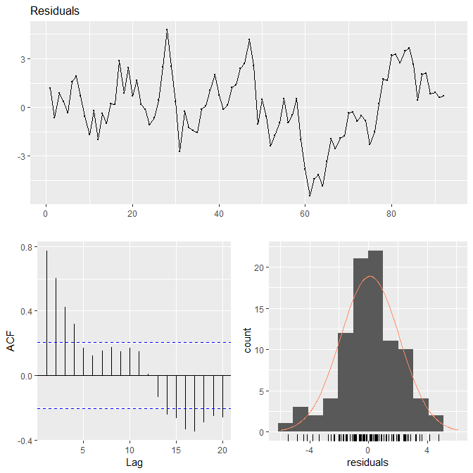
Compare this with the previous plot. So the actual challenge is estimating the discount factor. If we can solve this challenge we can build a robust algorithmic trading strategy based on it. One solution can be to avoid using the discount factor. We can build local level model, local linear trend model and the quadratic growth model and usu log likelihood to rank the three models and choose the model with the highest log likelihood for making the predictions.